The New Bond Regime: What Surging Sovereign Yields Mean for Global Markets

Global bond markets are undergoing a significant repricing of long-term borrowing costs. The U.S. 10-year Treasury yield recently touched 5.34%, its highest level since 2002. The UK 30-year gilt yield reached around 6.03%, its highest since 1998.

This is more than a conventional interest-rate cycle. It is a broader reset in the price of capital, particularly the cost of holding long-duration assets. Governments are running large fiscal deficits, inflation remains vulnerable to energy shocks, and corporations—particularly technology and AI companies—are competing with sovereign borrowers for long-term capital.

Why are global bond yields rising?

1. Fiscal borrowing, QT and the term premium

Governments are issuing increasingly large volumes of debt to finance fiscal deficits and refinance existing obligations. At the same time, the extraordinary support provided by Quantitative Easing (QE) has largely disappeared.

The Bank of England continues to reduce its gilt holdings through quantitative tightening (QT), while the Federal Reserve ended its balance-sheet runoff in December 2025. The important point is that central banks are no longer acting as the persistent, price-insensitive marginal buyers of government bonds that they were during the QE era.

A larger share of new issuance therefore has to be absorbed by private, price-sensitive investors. This can increase the term premium—the compensation investors demand for holding longer-duration bonds amid uncertainty about inflation, fiscal sustainability and future interest rates.

The pressure is compounded by the scale of U.S. borrowing. With U.S. national debt now above $40 trillion, persistent fiscal deficits are keeping Treasury issuance elevated, making the cost of refinancing increasingly important.

2. Inflation and “higher for longer”

Renewed energy-price pressures complicate the inflation outlook. Higher oil prices can feed into transportation, manufacturing and services costs, forcing markets to reassess how quickly central banks can cut rates.

3. Corporations are competing for capital

Governments are not the only borrowers. AI infrastructure, data centres and energy investment are creating substantial corporate demand for long-term capital. Five major hyperscalers—Alphabet, Amazon, Meta, Microsoft and Oracle—issued about $93 billion of bonds in 2025, versus an average of $35 billion annually in 2020–24; issuance had already reached roughly $132 billion by August 2026.

This reinforces the broader competition for long-duration capital: governments are borrowing heavily while corporations are simultaneously funding large-scale AI and infrastructure investment.

Why the reason for the yield rise matters

A bond yield rising because growth is accelerating is fundamentally different from a yield rising because investors are demanding compensation for inflation or deteriorating fiscal credibility.

The latter can create a much more difficult environment for financial assets because higher yields are accompanied by greater uncertainty about inflation, fiscal sustainability and the future path of interest rates.

What does this mean for equities?

Higher long-term yields increase the discount rate applied to future corporate cash flows, putting particular pressure on high-growth companies whose valuations depend heavily on distant earnings.

Higher bond yields also create greater competition for capital. When government securities offer materially higher returns, the equity risk premium can come under pressure.

At the same time, companies with significant debt face higher refinancing costs. Strong balance sheets, pricing power and sustainable free cash flow therefore become increasingly valuable.

This does not necessarily imply an equity-market collapse. Strong earnings can offset higher discount rates. But the environment becomes less forgiving: valuation expansion becomes harder and balance-sheet quality matters more.

Gold: the structural reserve-diversification trade

Gold faces a cyclical headwind from higher real yields and potentially a stronger dollar. But an increasingly important structural force is central-bank reserve diversification.

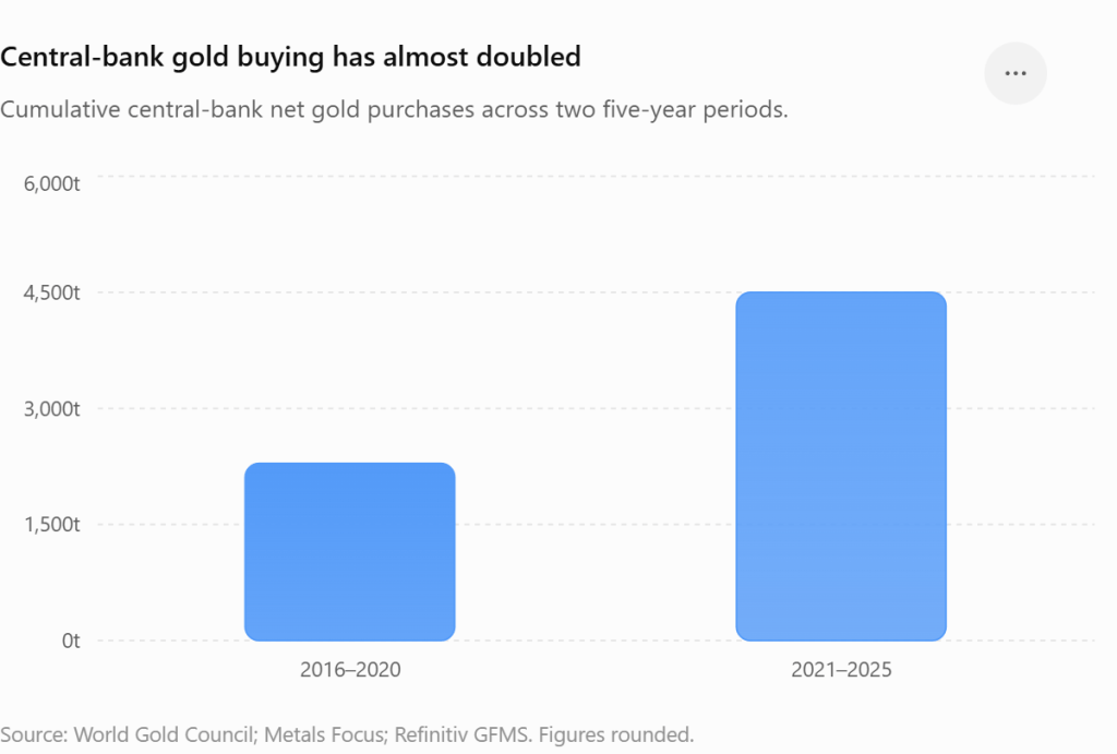
The change in official-sector buying over the past decade is striking:

PeriodCentral-bank gold purchases
2016–2020~2,290 tonnes
2021–2025~4,500 tonnes
Source: World Gold Council; Metals Focus; Refinitiv GFMS. Figures rounded.

Central-bank gold accumulation has therefore almost doubled over the past five-year period, highlighting the growing importance of gold in reserve diversification.

The direction of travel is equally important. The dollar’s share of global reserves has declined from 71% in 2000 and 66% in 2015 to around 57% today. At the same time, the World Gold Council’s 2026 survey found that 89% of reserve managers expect global central-bank gold holdings to increase over the next 12 months, while 83% expect gold’s share of reserves to rise over the next five years; 74% expect the dollar’s share to decline.

This does not mean central banks are abandoning the dollar or Treasuries. Rather, it points to incremental diversification away from concentrated dollar exposure and toward a more diversified reserve architecture.

That distinction matters in a world of rising sovereign debt. Gold is not another government’s liability and carries no direct sovereign or corporate counterparty risk. Higher real yields can remain a cyclical headwind, but persistent official-sector accumulation provides structural support.

Silver: cyclical weakness, structural demand

Silver is more economically sensitive than gold, so fears of a manufacturing slowdown can pressure it when yields rise. Yet its industrial role provides an important structural counterweight.

Silver is widely used in photovoltaic cells, electrification, grid infrastructure and electronics. The Silver Institute expects another global market deficit in 2026, although thrifting and substitution in solar technology are reducing silver usage per unit of capacity.

Thus, silver combines a cyclical industrial risk with structural demand from electrification and constrained supply—potentially limiting downside compared with previous bear markets, although its volatility remains much higher than gold’s.

Emerging markets: a tougher policy environment

Higher developed-market yields can pull capital toward safer, higher-yielding assets, pressure EM currencies and increase the local-currency burden of dollar-denominated debt.

EM central banks therefore face a difficult policy dilemma: cutting rates can support domestic growth but weaken currencies and worsen imported inflation, while maintaining higher rates can restrain domestic demand.

The impact will vary. Economies with stronger external balances, manageable foreign-currency debt and credible monetary frameworks should be better positioned.

India: resilient economy, nervous market

India enters this environment with important structural advantages: domestic growth, infrastructure investment, a large internal market and a comparatively strong banking system.

But economic resilience does not mean immunity from global financial-market stress.

The recent correction in Indian equities illustrates this distinction. Rising global yields, elevated crude prices and foreign selling have increased investor caution. India’s equity market can therefore undergo a meaningful valuation correction even while the underlying economy remains relatively strong.

However, India’s market structure has also changed. Domestic institutional and retail flows—particularly SIPs and pension-linked savings—provide an important counterweight to FPI selling. SIP contributions reached ₹32,297 crore in August 2026, demonstrating the scale of recurring domestic investment.

This does not create a hard valuation floor. But it can reduce the probability of the disorderly capital-flight dynamics seen in earlier emerging-market crises.

With U.S. Treasuries yielding above 5%, foreign investors face a much higher hurdle rate when allocating to relatively expensive emerging-market equities. Domestic investors, meanwhile, continue investing through local savings flows.

India could therefore experience an orderly phase of multiple contraction rather than a classic currency-and-market crisis.

The key vulnerability remains crude oil: sustained high prices could widen the current-account deficit, increase inflationary pressure and weaken the rupee.

The bigger investment message

The global financial system may be entering a regime in which the cost of duration matters much more than it did during the ultra-low-rate era.

Governments need to borrow heavily. Corporations are undertaking enormous capital-investment programmes. Central banks are no longer providing the same persistent demand for duration that characterised QE. Inflation remains vulnerable to energy and geopolitical shocks, while investors are demanding greater compensation for holding long-term assets.

The implications are therefore broader than simply “higher bond yields.”

Equity valuations face greater pressure, highly leveraged companies become more vulnerable, emerging markets face tighter financial conditions, while gold benefits from an increasingly important structural force—reserve diversification.

For India, the message is nuanced: economic resilience provides a buffer, domestic flows provide market depth, but the recent correction shows that investors remain nervous about the global cost of capital, oil prices and liquidity.

The emerging regime can therefore be summarised in one sentence:

The world is moving from an era of abundant cheap capital toward an era in which capital is more expensive, duration carries a higher premium, and reserve diversification matters more.

NVIDIA’s $500 Billion AI Bet: The Risk Investors Should Be Watching

AI infrastructure is entering a new phase: the financing phase.

On August 10, 2026, NVIDIA announced partnerships with Apollo, BlackRock, Blackstone, Brookfield, Goldman Sachs and KKR to help mobilize more than $500 billion of third-party capital over time for AI infrastructure.

The headline is enormous. But investors should look beyond it.

The more interesting story is what happens when AI infrastructure moves from a capex story to a financing story.

The real question is:

Can the infrastructure being financed today generate enough cash flow to justify the capital being deployed?

The mechanism is straightforward:

Capital → AI infrastructure → GPUs/accelerators → AI services → revenue → cash flow → investor returns and debt service.

NVIDIA benefits early in that cycle. The more difficult question comes later: Does the infrastructure generate sufficient economic returns?

NVIDIA: From Gaming GPUs to the AI Infrastructure Engine

NVIDIA’s transformation over the past decade is central to understanding this story.

What began primarily as a gaming GPU business has evolved into a computing platform increasingly centered on Data Center and AI.

The financial shift is striking.

In FY2016, Gaming revenue was $2.82 billion, versus $339 million from Data Center — Gaming was about 8.3 times larger. By FY2026, the relationship had completely inverted: Data Center generated $193.7 billion, versus $16.0 billion from Gaming — more than 12 times larger.

Over the decade, Data Center revenue expanded by roughly 570x, moving from less than 7% of NVIDIA’s revenue to nearly 90%.

This is more than a change in revenue mix.

NVIDIA is now deeply leveraged to the AI infrastructure cycle.

The Telecom Lesson: Lucent and Winstar

There is a useful historical precedent.

During the late-1990s telecom boom, Lucent Technologies provided Winstar Communications with a $2 billion credit facility, helping Winstar purchase Lucent equipment and expand its network. Winstar subsequently filed for Chapter 11 bankruptcy protection in 2001 as the telecom downturn intensified.

The lesson isn’t that NVIDIA is another Lucent. It is about financing infrastructure against expectations of future demand.

When demand grows as expected, financing accelerates expansion. When demand disappoints, the infrastructure remains — but the economics supporting the financing can change dramatically.

Risk #1: AI Monetization May Lag AI Capex

AI infrastructure investment is accelerating faster than the ultimate monetization of many AI applications.

Hyperscalers can spend billions today. But returns depend on customers eventually paying for AI services at sufficient scale and margins.

This creates a potential gap between:

AI capex today → AI cash flow tomorrow.

If utilization, pricing or enterprise adoption disappoints, infrastructure returns could fall even while AI demand remains strong.

AI can be transformative and an investment can still generate a poor return.

Risk #2: The Custom-Silicon Shift

The hyperscalers are increasingly developing their own silicon.

Google has its TPU family, Amazon has Trainium, and Meta is investing heavily in MTIA custom accelerators.

This is not necessarily an NVIDIA exodus. But custom silicon gives hyperscalers another option — and potentially greater control over the economics of AI compute.

NVIDIA’s CUDA ecosystem creates significant switching costs, particularly for enterprises, regional cloud providers and sovereign AI deployments already built around its software stack.

The investor question is:

What percentage of incremental AI compute will NVIDIA capture as custom silicon expands?

Risk #3: AMD and Intel Increase Competitive Pressure

AMD’s Instinct portfolio, including MI300X and MI350X, provides an alternative for high-performance AI workloads. Intel’s Gaudi 3 adds another option.

Neither company needs to displace NVIDIA to affect its economics. They only need to increase customer choice.

More alternatives can mean greater pricing pressure, stronger negotiating power for hyperscalers and potentially lower returns across the AI infrastructure stack.

Market growth and market economics are not the same thing.

Risk #4: Not All AI Infrastructure Has the Same Economic Life

AI factories contain different types of assets.

Land, grid connections, substations, cooling and physical infrastructure can have long useful lives and potentially retain value as scarce power-connected infrastructure.

Accelerators are different.

Their economic value is more exposed to technology cycles, performance-per-dollar improvements, compute pricing and utilization.

NVIDIA argues that AI compute can become an investable infrastructure asset, pointing to its broad customer base, software ecosystem and redeployability. It cites the A100, introduced in 2020, as hardware that remains in active commercial use six years later.

That creates an important counterpoint to the obsolescence argument.

The question is not simply whether the GPU will still work when the debt matures.

It is whether the GPU will retain enough economic value and cash-generating capacity throughout the financing period.

A GPU can remain operational while becoming less competitive, generating lower rental revenue or commanding a lower resale price.

That is economic obsolescence — and it matters when the equipment is part of a financed asset base.

The 25% Question

NVIDIA’s disclosure makes the financing structure even more interesting.

In its August 11 blog, NVIDIA states that in some cases it may provide residual-value support for up to 25% of an opportunity, assessed project by project.

This is not a blanket 25% guarantee.

But it indicates that, in selected transactions, NVIDIA may retain some exposure to residual-value risk.

The key equation becomes:

GPU utilization + compute pricing + residual value − financing costs = project economics

Risk #5: The Financing Flywheel Can Also Work in Reverse

Third-party financing can accelerate AI infrastructure deployment:

Capital → more AI factories → more compute → more AI capacity → more revenue potential.

But the reverse is also possible:

Lower utilization → weaker cash flow → tighter underwriting → higher financing costs → slower deployment.

Financing can therefore amplify both expansion and contraction.

The $500 billion headline should also not be interpreted as $500 billion of guaranteed demand for NVIDIA’s products. NVIDIA describes it as aggregate third-party capital that financing platforms are designed to mobilize over time.

So Who Carries the Risk?

The $500 billion is not a single $500 billion loan or $500 billion of NVIDIA debt. It represents aggregate third-party capital that financing platforms are designed to mobilize over time.

A useful way to think about the capital stack is as a risk waterfall, although the actual structure will vary by project:

Project / Customer Equity → Contractual or Residual-Value Support → Private Credit / Mezzanine → Senior Asset-Backed Financing

NVIDIA’s disclosed support mechanism is not equivalent to a blanket guarantee for the financing stack. It is project-specific, may cover residual value for up to 25% of an opportunity, and sits alongside independent underwriting.

If a project underperforms, project cash flows may fall short, equity returns may decline, credit providers face debt-service and recovery risk, and asset owners face utilization and residual-value risk.

Financing can redistribute risk across the capital structure. It does not eliminate it.

The ultimate question is:

Who absorbs the loss when utilization, pricing or residual values fall below underwriting assumptions?

What Investors Should Watch

1. AI monetization — Is AI revenue growing fast enough to support the capex cycle?

2. Compute utilization — Are expensive AI systems generating sufficient revenue per deployed accelerator?

3. Compute pricing — Are falling compute costs accelerating demand or compressing infrastructure returns?

4. Custom silicon — How quickly are hyperscalers shifting workloads toward internally designed chips?

5. Financing quality — Who provides the capital, what are the terms, and who bears the downside if cash flows or residual values disappoint?

The Investment Question Has Changed

The first phase of AI investing was about whether AI would create demand for computing.

The next phase is about whether the economics of that computing justify the capital being deployed.

NVIDIA has been one of the principal commercial beneficiaries of the AI infrastructure buildout. But as financing scales, downstream economics become increasingly important.

The telecom lesson remains relevant:

Infrastructure demand can be real. Technology adoption can be real. And financing can still get ahead of the economics.

The $500 billion question is therefore not simply:

How much capital can AI attract?

It is:

How much sustainable cash flow will that capital generate — and who carries the downside if it doesn’t?

Reference: NVIDIA Blog August 11, 2026 – “NVIDIA AI Factory Compute Is Becoming an Investable Asset Class” .


Understanding Risk to Reward in Trading

Before entering any trade, an investor should ask two simple questions:

How much can I lose? And how much can I potentially make?

This is where Risk : Reward becomes important.

Risk : Reward helps us compare the potential loss from a trade with its potential gain. It does not predict whether a trade will be successful, but it helps us determine whether the potential reward justifies the risk we are taking.

How to Calculate Risk : Reward

Risk : Reward can be expressed as:

Risk : Reward = Potential Loss : Potential Gain

For example, if you are risking ₹10 to potentially make ₹25:

₹10 : ₹25 = 1 : 2.5

This means you are risking ₹1 to potentially make ₹2.50.

For equity trading, a Risk : Reward of 1:2.5 or better is often considered a desirable general guideline, given the relatively higher volatility and risk associated with equities.

However, 1:2.5 is not a rule. A favorable Risk : Reward alone does not make a trade attractive. The probability of reaching the target, the quality of the setup, and proper risk management are equally important.

Risk : Reward vs Probability

This is an important distinction.

Risk : Reward tells you how much you could potentially gain relative to what you are risking. Probability tells you how likely that outcome may be.

For example, a trade offering a 1:10 Risk : Reward may look extremely attractive, but if the target is very difficult to reach, the probability of success could be low.

Therefore, investors should consider both Risk : Reward and the probability of achieving the target rather than focusing only on the ratio.


A Case Study of Sheela Foam

Let’s understand the concept with the help of a technical example of Sheela Foam.

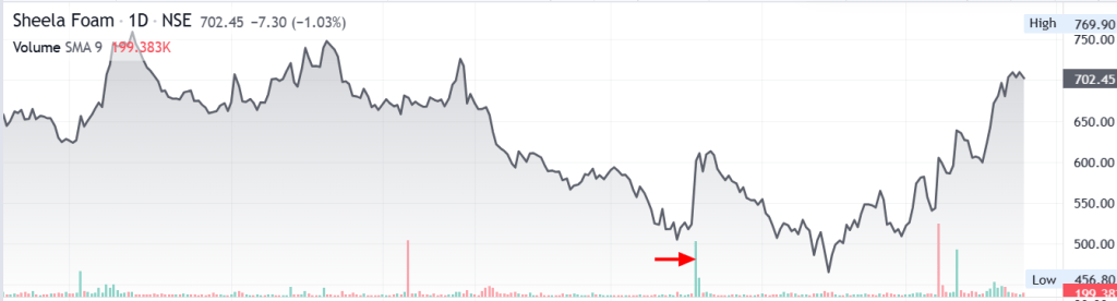
Sheela Foam — Daily NSE Price Chart
Chart Source : Moneycontrol

What Does the Chart Tell Us?

1. Triple-top formation

Sheela Foam formed a potential triple-top pattern around the ₹830 level (See Red Arrow in the chart above).

On July 13, August 4 and August 5, the stock attempted to cross and sustain above ₹830 but failed, indicating that ₹830 was acting as a strong resistance zone.

2. Breakdown below support

Following the June 26 quarterly results, the stock witnessed profit booking and subsequently broke below the ₹730–₹735 support zone.

This zone had been tested around July 2, July 8 and July 22 (See Blue Arrow in the chart above).

The breakdown occurred on higher trading volume, suggesting that selling pressure was increasing.

When a stock breaks an important support level on higher volume, it can indicate that more market participants are willing to sell at lower prices.

3. Double-bottom formation

After the breakdown, the stock tested a low of approximately ₹662 twice, on August 10 and August 18, forming a potential double-bottom pattern (See Green arrow in the chart above).

Interestingly, these tests occurred on declining volumes, suggesting that selling pressure was weakening.

The stock also remained just above its 200-Day Moving Average (DMA) of ₹655.99, providing another technical reference point.


Now Let’s Calculate the Risk

Suppose an investor considers a hypothetical entry price of approximately ₹666.

A stop-loss (SL) is placed at ₹660, below the ₹662 double-bottom support.

Therefore:

Entry Price = ₹666

Stop-Loss = ₹660

Potential Risk = ₹666 − ₹660 = ₹6 per share

In simple terms:

You are risking ₹6 per share.

The next question is:

How much could you potentially make?


Potential Rewards

TargetTarget PricePotential GainWhy This Target?Risk : Reward
Target 1₹717₹51Previous relief-rally high of ₹717 made on August 121 : 8.5
Target 2₹735₹69Previous ₹730–₹735 support zone, which could now act as resistance1 : 11.5
Target 3₹832₹166Previous resistance zone around ₹830–₹8321 : 27.7

Why can previous support become resistance?

The earlier ₹730–₹735 level acted as support. After the stock broke below it, this same zone may become resistance.

One reason is that investors who bought around this level may look to exit when the price returns to their purchase zone, creating additional selling pressure.


Putting It All Together

Target 1

The ₹6 → ₹51 → 1:8.5 Story

🔵 Entry: ₹666
🔴 Stop-Loss: ₹660
🎯 Target 1: ₹717

Potential Risk:
₹666 − ₹660 = ₹6

Potential Gain:
₹717 − ₹666 = ₹51

Therefore:

₹6 Risk → ₹51 Potential Reward

₹6 : ₹51 = 1 : 8.5

In simple terms:

For every ₹1 being risked, there is a potential reward of ₹8.50.

This is the essence of Risk : Reward.

Target 2

Potential gain = ₹735 − ₹666 = ₹69

Therefore:

₹6 : ₹69 = 1 : 11.5

You are risking ₹1 to potentially make ₹11.50.

Target 3

Potential gain = ₹832 − ₹666 = ₹166

Therefore:

₹6 : ₹166 = 1 : 27.7

You are risking ₹1 to potentially make ₹27.70.


What Does This Tell Us?

Based purely on the hypothetical entry, stop-loss and targets, the setup offers a potentially favorable Risk : Reward profile.

However, there is an important point to remember:

A higher Risk : Reward does not necessarily mean a better trade.

Target 3 offers a very attractive 1:27.7 Risk : Reward, but it is considerably farther away and may therefore have a lower probability of being achieved than Target 1.

The purpose of Risk : Reward analysis is not to predict the future with certainty.

It is to ensure that:

The potential reward is sufficiently large relative to the amount being risked.

So, don’t simply look for the highest Risk : Reward ratio.

Instead, consider:

Risk + Reward + Probability

A realistic target with a reasonable probability of achievement can be more useful than an extremely distant target with a very low probability of being reached.


Key Takeaway

Before entering a trade, don’t just ask:

“How much can I make?”

Also ask:

“How much can I lose if I am wrong?”

In this example, the hypothetical trade risks ₹6 per share for a potential gain of ₹51 at Target 1, resulting in a 1:8.5 Risk : Reward.

That is significantly better than the commonly used 1:2 or 1:2.5 guideline.

But remember:

Risk : Reward is only one part of the decision-making process.

A sound trading setup should ideally combine:

  • A clearly defined entry
  • A logical stop-loss
  • Realistic price targets
  • Favorable Risk : Reward
  • A reasonable probability of achieving the target
  • Disciplined execution

The objective is not simply to find trades with the highest Risk : Reward. It is to find trades where the potential reward, probability and risk are reasonably aligned.


Disclaimer

This illustration is intended solely to explain the concept of Risk : Reward using a technical example. It should not be considered a stock recommendation or investment advice. Readers should conduct their own research and due diligence and consider their individual risk appetite before making any investment decisions.

Disclosure

The author holds a position in Sheela Foam and therefore has a financial interest in the stock discussed in this article.


Understanding the Delivery Ratio: Separating Investor Conviction from Market Noise

Learn how to use price action, trading volume, and delivery ratio together to identify accumulation, distribution, and high-conviction market moves.

Why do some stocks rebound sharply after a steep fall, while others continue to decline?

Price and trading volume provide part of the answer, but they don’t reveal who is actually buying or selling. This is where the Delivery Ratio becomes a valuable indicator. It helps investors distinguish between short-term speculative trading and genuine investment activity, offering deeper insight into the conviction behind market moves.

Understanding Delivery Ratio

When analysing stocks, most investors focus on price movements and trading volume. While these indicators provide valuable insights, they don’t reveal the true intent behind market activity.

This is where the Delivery Ratio becomes an important tool.

The delivery ratio helps investors understand whether trading activity is driven by genuine investment interest or short-term speculation. By combining delivery ratio with price and volume analysis, investors can better judge the strength and sustainability of a market trend.


What is the Delivery Ratio?

The delivery ratio is the percentage of shares traded during a day that are actually transferred to buyers’ demat accounts for settlement.

In simple terms, it tells us how many shares were bought for holding rather than for intraday trading.

Formula

Delivery Ratio = (Deliverable Quantity ÷ Total Traded Quantity) × 100

Example

Suppose a stock trades 10 lakh shares during the day.

  • Shares traded: 10,00,000
  • Shares delivered to buyers: 7,50,000

Delivery Ratio = (7,50,000 ÷ 10,00,000) × 100 = 75%

This means that 75% of the traded shares were purchased for delivery, while the remaining 25% were likely intraday trades.


Why is the Delivery Ratio Important?

The delivery ratio provides insight into the quality of trading volume.

Two stocks may record identical trading volumes, but the one with the higher delivery ratio generally indicates stronger investor participation and conviction.

It helps investors:

  • Distinguish between long-term investing and short-term speculation
  • Identify possible accumulation or distribution by large investors
  • Confirm the strength of a price breakout or breakdown
  • Filter out false signals created by speculative trading

Interpreting the Delivery Ratio

1. High Volume + Low Delivery Ratio

A large number of shares are traded, but only a small percentage are taken for delivery.

What does it indicate?

  • Most of the trading activity is likely intraday or speculative.
  • Traders are buying and selling shares within the same trading session.
  • High trading volume may create excitement, but it does not necessarily reflect strong investor conviction.
  • Such price movements are often driven by short-term sentiment and can reverse quickly.

Example

A stock trades 1 crore shares, but only 20 lakh shares are delivered.

Delivery Ratio = 20%

This indicates that most of the day’s activity was speculative.

Key Interpretation

High trading activity + Low investor commitment = Speculative movement


2. High Volume + High Delivery Ratio

A large number of shares are traded, and a significant percentage are taken into investors’ demat accounts.

What does it indicate?

  • Indicates strong buying or selling conviction.
  • Investors are willing to hold their positions instead of exiting on the same day.
  • If accompanied by a price increase, it may indicate accumulation by institutions or long-term investors, making the uptrend more reliable.
  • If accompanied by a price decline, it may suggest distribution or sustained selling pressure.

Example

A stock trades 1 crore shares, and 75 lakh shares are delivered.

Delivery Ratio = 75%

This suggests that investors are willing to hold the stock.

Key Interpretation

High trading activity + High investor commitment = Strong conviction and a more sustainable trend


3. Low Volume + High Delivery Ratio

Trading volume is relatively low, but a high percentage of the traded shares are taken for delivery.

What does it indicate?

  • Suggests quiet accumulation by long-term investors.
  • Although overall participation is low, those buying the stock intend to hold it.
  • Often observed during the early stages of an uptrend or while informed investors gradually build positions.
  • The stock may remain range-bound until broader market participation increases.
  • If the stock later breaks out with a sharp increase in volume, it strengthens the bullish case.

Example

A stock trades 10 lakh shares, and 8 lakh shares are delivered.

Delivery Ratio = 80%

This indicates that most buyers intend to hold the stock.

Key Interpretation

Low trading activity + High investor commitment = Quiet accumulation


4. Low Volume + Low Delivery Ratio

Trading volume is low, and only a small percentage of shares are taken for delivery.

What does it indicate?

  • Reflects limited interest from both investors and traders.
  • Neither long-term investors nor speculative traders are actively participating.
  • Stocks with this combination often move sideways with low liquidity.
  • Price movements generally lack momentum until fresh buying interest emerges.

Example

A stock trades 10 lakh shares, but only 2 lakh shares are delivered.

Delivery Ratio = 20%

This indicates weak participation from the market.

Key Interpretation

Low trading activity + Low investor commitment = Weak market interest

Disclaimer: The following case study is based on publicly available trading data and represents one possible interpretation of market behaviour. No single indicator can conclusively prove institutional buying or selling. Delivery ratio should always be analysed alongside price action, trading volume, and broader market context.

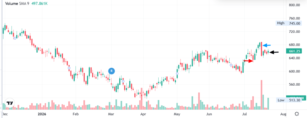
Case Study : Analyzing Delivery Ratio – Healthcare Global Enterprises (HCG)

HCG Graph source : Moneycontrol.com

Red arrow – 8th July (-2.0% Price drop / Delivery 89.1%)

Blue arrow : 15th July (-5.8% Price drop / Delivery 86.7%)

Black arrow : 21st July (Delivery 94.4%)

How Delivery Ratio Revealed Institutional Accumulation

The table below shows the relationship between price movement, trading volume, and delivery percentage over multiple trading sessions.

DateClosing Price (₹)Day Change (%)Traded QuantityDelivered QuantityDelivery (%)VWAP (₹)
21 Jul 2026661.25+1.1%9,73,1999,18,32294.4%655.65
20 Jul 2026653.70-0.3%68,74939,79057.9%655.78
17 Jul 2026655.85-0.6%75,51144,22258.6%655.88
16 Jul 2026660.10+2.0%6,35,8805,47,49286.1%—
15 Jul 2026646.85-5.8%19,51,00016,91,51786.7%—
14 Jul 2026686.35+1.1%1,38,00877,04755.8%682.69
13 Jul 2026678.85+1.9%1,48,46484,65757.0%676.38
10 Jul 2026666.40+2.1%2,80,6341,71,32061.0%665.20
09 Jul 2026652.70+2.9%1,12,11058,29752.0%—
08 Jul 2026634.50-2.0%5,67,3905,05,54489.1%—
07 Jul 2026647.65-0.8%4,07,0403,32,55181.7%—
06 Jul 2026652.60-0.3%74,84040,48854.1%—
03 Jul 2026654.80+0.9%1,14,87069,15160.2%—
02 Jul 2026649.00+2.4%2,12,7601,19,14556.0%—

Key Takeaways From the Data:

One trading day stands out:

DatePrice ChangeTraded QuantityDelivery %
15 Jul 2026-5.8%19.5 lakh shares86.7%

At first glance, many retail investors would consider this a bearish signal because the stock witnessed a sharp fall of nearly 6%.

However, a deeper analysis tells a different story.


Looking Beyond the Price

A sharp decline accompanied by very high trading volume usually attracts attention.

Many retail traders interpret this as a breakdown and panic sell.

Professional investors, however, often view these situations differently.

Periods of panic selling create liquidity—allowing institutions to accumulate large quantities of shares without significantly pushing prices higher.


Why This Data Suggests Accumulation

On 15 July, the stock experienced:

  • Sharp price correction (-5.8%)
  • Exceptionally high trading volume
  • Very high delivery percentage (86.7%)

The high delivery percentage indicates that most of the traded shares were actually transferred to investors’ demat accounts rather than squared off as intraday trades.

This suggests that buyers were willing to hold the shares despite the sharp fall.

More importantly, the subsequent trading sessions strengthen this interpretation.

Following the decline:

  • Delivery percentages remained consistently high.
  • The stock stabilized near the ₹645–₹655 zone.
  • Within a few trading sessions, the price recovered to ₹661.25, while delivery percentage increased further to 94.4%.

This combination suggests that the selling pressure was gradually absorbed by committed buyers.


Institutional Buying Often Happens During Fear

Institutional investors rarely chase stocks after a strong rally.

Instead, they often prefer buying during periods of fear when liquidity is abundant.

Rather than placing aggressive market orders, they may place large passive buy orders around important support levels.

As panic sellers exit, institutions quietly absorb the available supply.

Once the excess selling pressure is exhausted, prices often stabilize and recover.

This appears consistent with the pattern observed around the ₹645–₹655 price zone in this example.


Key Learning

A falling price combined with a high delivery percentage does not automatically mean a stock is bullish.

Instead, it indicates strong conviction among market participants.

To determine whether it represents accumulation or distribution, investors should analyse:

  • Subsequent price action
  • Trading volume
  • Delivery percentage over several sessions
  • Key support and resistance levels

In this case, the subsequent recovery in price and consistently high delivery percentages support the view that the decline was likely an accumulation phase rather than a continuation of bearish momentum.


Investor Takeaway

Price tells you what happened.

Volume tells you how much activity took place.

Delivery ratio tells you how much of that activity resulted in actual ownership.

When all three indicators are analysed together, they provide a much clearer picture of market sentiment than any one indicator alone. This is why experienced investors use the combination of price, volume, and delivery ratio to distinguish between panic selling, speculative trading, accumulation, and distribution.


Quick Takeaway

ScenarioWhat It SuggestsInvestor Focus
High Volume + High DeliveryStrong investor convictionConfirm trend with price action
High Volume + Low DeliveryMostly speculative activityBe cautious of false breakouts
Low Volume + High DeliveryQuiet accumulationMonitor for volume expansion and breakout
Low Volume + Low DeliveryWeak market interestAvoid until participation improves

Important Points to Remember

  • A high delivery ratio does not always guarantee that the stock will rise. It simply indicates stronger holding interest.
  • A low delivery ratio does not always imply weakness. It may simply reflect active intraday trading.
  • Always interpret the delivery ratio in conjunction with price movement and trading volume.
  • The delivery ratio is most useful when analysed over multiple trading sessions, rather than a single day.
  • Compare the delivery ratio with the stock’s historical average to identify unusual accumulation or distribution.

Common Mistakes Investors Make

  • Assuming a high delivery percentage is always bullish.
  • Looking at only one day’s delivery data instead of analysing multiple sessions.
  • Ignoring price action while interpreting delivery.
  • Ignoring overall market trend.
  • Taking trading decisions solely based on delivery ratio.

Delivery Ratio Checklist

Before taking a trading or investing decision, ask yourself:

✅ Is the stock trading near an important support or resistance?

✅ Has volume increased significantly?

✅ Is the delivery ratio above its historical average?

✅ Is price confirming accumulation or distribution?

✅ Is the broader market supporting the move?

If the answer is Yes to most of these questions, the delivery ratio provides much stronger confirmation.


Final Thoughts

Successful investing isn’t about relying on a single indicator—it’s about combining multiple pieces of evidence.

  • Price tells you where the market is moving.
  • Volume tells you how much participation there is.
  • Delivery Ratio tells you how much conviction exists behind that participation.

When all three point in the same direction, investors gain greater confidence in identifying accumulation, distribution, breakouts, and potential trend reversals.

“Price creates the story, Volume gives it credibility, and Delivery Ratio reveals the conviction behind it.”

Use the delivery ratio not as a standalone signal, but as a confirmation tool alongside price action, trading volume, support and resistance, and broader market trends. Over time, this disciplined approach can help you make more informed and confident investment decisions.


Understanding the Importance of Trading Volume in Stock Analysis

While analyzing stock price movements, the primary focus is usually on price action. However, trading volume is equally important because it validates the strength and reliability of a price move.

Volume refers to the total number of shares traded on the stock exchange during a particular trading session.

Why is Volume Important?

1. Trend Confirmation

Volume confirms the strength of a price trend. A rise in price accompanied by increasing volume indicates strong buying interest, making the trend more reliable.

2. Breakout Confirmation

When a stock breaks above a key resistance level on high volume, it confirms strong market participation. Such breakouts are more likely to sustain than those occurring on low volume.

3. Breakdown Confirmation

When a stock breaks below a key support level on high volume, it indicates strong selling pressure. High-volume breakdowns are generally more reliable and often signal further downside, while low-volume breakdowns are more prone to failure.


Interpreting Volume in Technical Analysis

1. Bullish Trend Confirmation – Rising Price on High Volume

  • Indicates strong buying interest from investors and traders.
  • Confirms that the uptrend is supported by conviction and is more likely to continue.
  • High trading volume validates the breakout, increasing the probability of a sustained uptrend.
High volume confirms the breakout, increasing the probability of a sustained uptrend
Graph source: Moneycontrol

2. Bearish Volume Divergence – Rising Price on Low Volume

  • Indicates weak buying participation despite rising prices.
  • The rally lacks broad market participation and institutional support.
  • The price may continue rising temporarily, but the move is less reliable and more vulnerable to a reversal.

Interpretation:
Ideally, rising prices should be accompanied by increasing volume. When prices rise while volume remains low or declines, it is known as bearish volume divergence, signalling that the uptrend may be losing strength.

3. Bearish Trend Confirmation – Falling Price on High Volume

  • Indicates strong selling pressure as investors and traders exit the stock.
  • Confirms that the downtrend is supported by conviction.
  • High selling volume validates the breakdown, increasing the probability of further downside.
High selling volume confirms the breakdown, increasing the probability of further downside
Graph source: Moneycontrol

4. Bullish Volume Divergence – Falling Price on Low Volume

  • Indicates limited selling interest despite falling prices.
  • The decline lacks strong selling conviction.
  • Selling pressure may be weakening, increasing the possibility of price stabilization or a reversal if buyers return.

Interpretation:
When prices fall while trading volume decreases, it is known as bullish volume divergence. This suggests that sellers are losing momentum and the downtrend may be approaching exhaustion. Traders often wait for additional confirmation before expecting a reversal.

Key Takeaway

Price tells you what is happening. Volume tells you how strongly the market believes in that move.

A price move supported by high trading volume is generally more reliable than one occurring on low volume. Successful traders combine price action and volume analysis to:

  • Confirm market trends.
  • Validate breakouts and breakdowns.
  • Identify bullish and bearish volume divergences.
  • Avoid false trading signals.

Golden Rule

Price shows the direction. Volume confirms the conviction.

Rethinking the Rule of 100: A Modern Approach to Investment Risk

Rethinking the Rule of 100

A Story to Begin With

Two investors walk into the same financial planning office.

The first is 28 years old, earning a decent salary but juggling a home loan, car EMI, and plans for a child’s education. The second is 62, recently retired, debt-free, with accumulated savings and a steady pension.

According to the Rule of 100, the younger investor should aggressively invest in equities, while the older one should sharply reduce stock exposure. But when you look at their real financial lives, the picture feels counterintuitive. The younger investor cannot afford large losses, while the retired investor may actually have the stability to ride out market volatility.

This disconnect raises an important question:
Should age alone determine how much investment risk you take?

That question sits at the heart of this article.


The Rule of 100 – Asset Allocation by Age

When it comes to investing, one of the most common questions people ask is:
How much should I invest in equities and how much in safer assets?

To simplify this decision, financial planners have long relied on age-based formulas—the most popular being the Rule of 100.

At first glance, the rule seems logical and easy to follow. But does it truly reflect how real people earn, save, and spend today? Let’s take a closer look.


What Is the Rule of 100?

The Rule of 100 is a basic guideline used to determine asset allocation based on age.

Formula:
100 − Your Age = Percentage of your portfolio invested in equities

The remaining portion is allocated to bonds, debt instruments, or other relatively low-risk assets.

Simple Examples

  • Age 30
    • 70% in stocks
    • 30% in bonds/debt
  • Age 50
    • 50% in stocks
    • 50% in bonds/debt

The Logic Behind the Rule

The rule is built on a straightforward assumption:
risk tolerance declines with age.

Younger investors are expected to have:

  • Longer investment horizons
  • More time to recover from market downturns

Older investors, on the other hand, are assumed to:

  • Prefer stability over growth
  • Focus on capital preservation and steady income

This thinking made sense decades ago—but markets, careers, and lifespans have changed.


Why the Rule Evolved: Rule of 110 and Rule of 120

As life expectancy increased and inflation became a bigger threat, financial advisors began adjusting the formula.

Rule of 110

110 − Age = Equity allocation

  • Age 30 → 80% equities
  • Age 50 → 60% equities

This version recognizes that:

  • People are working longer
  • Retirement needs are larger
  • Equity growth is crucial to beat inflation

Rule of 120

120 − Age = Equity allocation

  • Age 30 → 90% equities
  • Age 50 → 70% equities

This rule is typically suggested for investors with higher risk tolerance or those relying heavily on equity markets for long-term wealth creation.

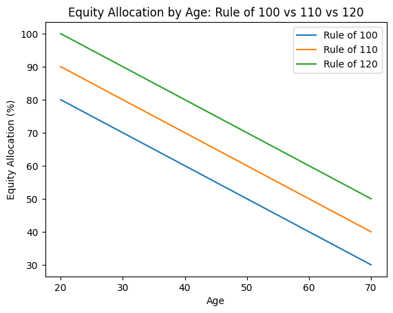
A comparison of Rule of 100 vs Rule of 110 vs Rule of 120 is shown in the chart below:

What the Chart Shows

  • X-axis: Investor age
  • Y-axis: Suggested equity allocation (%)

Three declining lines represent:

  • Rule of 100 (most conservative)
  • Rule of 110 (moderate)
  • Rule of 120 (most aggressive)

Key Takeaways:

  • All three rules reduce equity exposure linearly with age
  • The difference between rules becomes more pronounced at younger ages
  • Even at age 60–70, Rule of 120 still suggests meaningful equity exposure, reinforcing the inflation-risk argument

The Big Problem With All These Rules

Despite their popularity, the Rule of 100, 110, and 120 share one major flaw:

They assume age alone determines risk capacity.

In reality, age tells only part of the story.


A Contrarian Perspective: When the Rule Breaks Down

Younger Investors Aren’t Always Risk-Takers

Many young investors face:

  • Lower incomes and limited savings
  • Home loans, car EMIs, and education expenses
  • Small emergency buffers

For them, a sharp market fall can cause real financial stress. Even though time is on their side, their ability to absorb losses may be limited. In such cases, aggressive equity exposure can do more harm than good.

Older Investors May Have Higher Risk Capacity

Ironically, many older or retired investors:

  • Are free from major financial obligations
  • Have accumulated wealth, pensions, or rental income
  • Can emotionally handle short-term volatility

For them, maintaining meaningful equity exposure may actually be necessary to protect purchasing power against inflation.


The Real Question: Risk Tolerance or Risk Capacity?

This is where most age-based rules fall short.

  • Risk tolerance is how comfortable you feel with volatility
  • Risk capacity is whether your finances can survive a downturn

Risk capacity depends far more on:

  • Cash flows
  • Liabilities
  • Financial security
  • Emergency reserves

—not just your age.


Final Thoughts

The Rule of 100 and its modern variations are useful starting points, not formulas to follow blindly.

Smart asset allocation requires balancing:

  • Age
  • Income stability
  • Financial responsibilities
  • Long-term goals
  • The ability—not just the willingness—to take risk

In investing, simplicity helps.
But context matters even more.


What Do You Think?

  • Should age alone determine how much risk an investor takes?
  • Have your financial responsibilities increased or reduced your ability to invest in equities?
  • For younger investors with EMIs, is aggressive equity allocation practical—or risky?
  • Should retired investors reduce equity exposure simply because of age?
  • Which matters more: risk tolerance or risk capacity?
  • Do you follow the Rule of 100 (or 110/120), or have you created your own approach?

👉 Share your views—your experience may help others rethink how they invest.


The Magnificent 7: Are AI Stocks Setting Up for a Bubble?

Overview

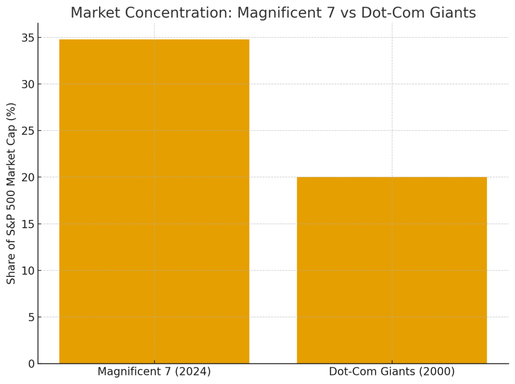
As of late 2024, the Magnificent 7 — Alphabet (Google), Amazon, Apple, Meta Platforms, Microsoft, Nvidia, and Tesla — collectively account for $16 trillion of the S&P 500’s $46 trillion total market capitalization.
This means these seven companies alone represent 34.8% of the entire index, a massive increase from about 10% in 2014.

For historical context, even during the dot-com bubble of 2000, the largest tech companies never exceeded 20% of the S&P 500. Today’s concentration level is therefore unprecedented.

Over the recent years, the heavy weighting of AI-focused companies has been a major driver of the S&P 500’s growth. This dependence has led many analysts to warn of a potential AI-driven valuation bubble and the risk of a sharp correction if expectations disappoint.

Risk of an AI Bubble Bursting

1. Valuation Risk

AI-focused companies are increasingly trading at valuations that far exceed their underlying fundamentals, echoing patterns seen during the Dot-Com era. For example, Palantir reported $1.18 billion in Q3 2025 revenue and is projecting around $4.40 billion for the full year. Yet its market capitalisation surged to nearly $450 billion, implying a valuation of 115–120× sales—levels typically associated with speculative excess rather than sustainable financial performance. This disconnect between valuation and fundamentals heightens the risk of sharp corrections if anticipated growth fails to materialize.

Many analysts argue that valuations are pricing in hyped future revenues, not current financial performance or realistic near-term applications of AI.

2. Capex vs. Actual Returns

Big Tech is expected to invest $5 trillion on AI-related infrastructure — data centers, chips, model training, and energy facilities.

However, the return profile does not yet justify this scale of investment:

  • Only around 5% of businesses currently use AI in full production environments.
  • Productivity gains remain slow and uneven.
  • Many AI tools still lack clear monetization paths.

This mismatch heightens the risk that expected AI-driven profits may not materialize soon enough to justify the massive capital outlay.

3. Rising Debt Financing

Despite being historically cash-rich, AI-focused tech giants have been taking on large amounts of debt to finance data-center expansion.

For example:

  • Oracle reported $124 billion in total obligations (including operating lease liabilities) as of Nov 2025 — up from $89 billion a year earlier.
  • Weak earnings combined with rising debt prompted S&P and Moody’s to revise Oracle’s credit outlook to negative.

Analysts see parallels to the dot-com era, when companies overborrowed to fund speculative, unproven technologies. If AI revenues lag, these debt loads could rapidly become unsustainable.

4. “Circular” Investment and Revenue Deals

An emerging concern is the rise of vendor-financed growth loops within the AI ecosystem.

A notable example involves:

  • Nvidia, which committed up to $100 billion in staged investments into OpenAI, contingent on the deployment of new AI infrastructure (e.g., gigawatts of data-center capacity).
  • OpenAI then uses the capital to purchase Nvidia chips, creating a circular flow of investment → purchase → revenue.

Analysts and regulators have pointed out that this model may artificially inflate demand and revenue, echoing vendor-financing practices seen in earlier speculative periods.

5. Concentration Risk in the S&P 500

With the Magnificent 7 making up nearly one-third of the total S&P 500, the broader market’s stability is increasingly tied to the performance of a small cluster of AI-centric companies.

A synchronized decline in these firms — due to AI monetization delays, regulatory pressure, competitive threats, or earnings disappointments — could:

  • Trigger broad market corrections
  • Mirror the systemic tech collapse of 2000
  • Reduce retirement savings, given heavy household exposure to index funds
  • Increase volatility across global equity and credit markets

The S&P 500’s dependence on a single technological narrative — AI dominance — heightens systemic vulnerabilities.


Summary

The rapid rise of AI has created unprecedented concentration within the S&P 500. While AI has transformative potential and the Magnificent 7 possess stronger fundamentals than the tech leaders of 2000, valuation excesses, massive capex commitments, rising debt, circular revenue arrangements, and extreme index concentration have raised concerns about a potential AI bubble.

If AI growth and monetization fall short of current expectations, the resulting correction could echo — or potentially exceed — the impact of the dot-com crash.

How to use RSI for Trading Success

Relative Strength Index (RSI)


A momentum indicator developed by J. Welles Wilder Jr. (1978) that measures the speed and magnitude of price changes. Traders use RSI to identify whether a stock is overbought or oversold.

RSI Scale

RSI moves between 0 and 100.

RSI Formula (Simple Version)

  • RS = Average Gains / Average Losses
  • RSI = 100 – [100 / (1 + RS)]

(You don’t usually need to calculate it manually—charting tools do it automatically.)

How to Read RSI

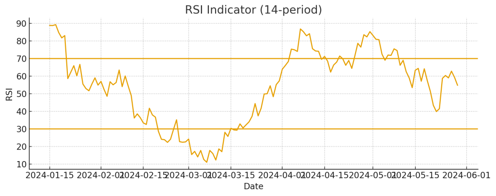
Overbought (RSI > 70)

  • An RSI above 70 suggests that the asset may be overbought, indicating a potential price correction.

Oversold (RSI < 30)

  • An RSI below 30 suggests the asset may be oversold, indicating a possible rebound.

Example Chart Explanation

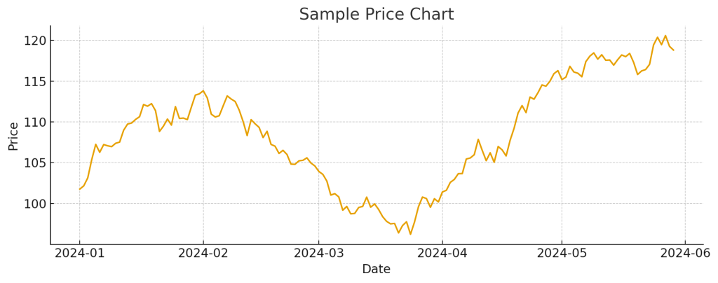
1. Price Chart

(shows the stock’s price movement over time.)

2. RSI Chart

(shows RSI oscillating between 0 and 100 with reference lines at 30 and 70.)

Overbought Example

When RSI rises above 70:

  • Momentum is strong but may be overstretched.
  • When RSI turns back below 70, the price often slows down or pulls back.

Oversold Example

When RSI falls below 30:

  • Indicates strong downside pressure.
  • When RSI rises above 30, price often stabilizes or rebounds.

How Traders Use RSI

  1. Entry Signal (Buy) : RSI crosses above 30 → possible buying opportunity.
  2. Exit Signal (Sell) : RSI crosses below 70 → possible selling signal.
  3. Trend Reversals (Divergence) Traders watch for differences between price movement and RSI movement:
    • Bullish Divergence:
      Price makes lower lows, but RSI makes higher lows.
      → Suggests a potential upward reversal.
      → Buy when RSI crosses above 30.
    • Bearish Divergence:
      Price makes higher highs, but RSI makes lower highs.
      → Suggests a potential downward reversal.
      → Sell when RSI crosses below 70.

Limitations

  • RSI can stay overbought or oversold for long periods during strong trends.
  • It may give false signals in sideways or choppy markets.
  • Works best when combined with price action, moving averages, MACD, or volume confirmation.

Conclusion

The RSI is a simple yet powerful indicator that helps traders understand momentum and identify potential turning points in the market. While it provides helpful signals for entries, exits, and trend reversals, it should not be used alone. Combining RSI with other technical tools and overall market context leads to more reliable and confident trading decisions.


Understanding Moving Averages in Trading

Moving Average (MA)

A moving average represents the average price of a security over a specific period, helping traders smooth out short-term price fluctuations and identify overall trends.

Types of Moving Averages

TypePeriod CoveredUsageTrend Focus
200-Day Moving Average (200-DMA)Last 200 trading daysLong-term trend identificationBroad market direction
50-Day Moving Average (50-DMA)Last 50 trading daysShort- to intermediate-term analysisRecent price momentum

How to Interpret a Moving Average

Golden Cross (Bullish Signal)

Definition:
Occurs when the 50-DMA crosses above the 200-DMA.

Interpretation:
→ Signals a bullish trend, indicating potential long-term upward momentum.
The crossover shows that short-term momentum is overtaking long-term averages, suggesting renewed market strength.

Confirmation:
Traders look for increasing trading volumes or other indicators (like RSI or MACD) to validate the uptrend.

Death Cross (Bearish Signal)

Definition:
Occurs when the 50-DMA crosses below the 200-DMA.

Interpretation:
→ Signals a bearish trend, indicating potential long-term downward momentum.
This suggests that short-term weakness is overtaking long-term support levels.

Confirmation:
Traders often seek validation through
• A break of key support levels
• Declining trading volumes
• Other bearish indicators

Example: Golden Cross – Northern ARC Capital Ltd

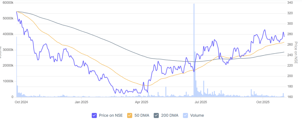
Northern ARC Capital Ltd (Chart source : https://www.screener.in)

In the chart above:

  • The blue line represents the price movement of the stock on NSE.
  • The orange line is the 50-Day Moving Average (50-DMA) — short- to mid-term trend indicator.
  • The grey line is the 200-Day Moving Average (200-DMA) — long-term trend indicator.
  • The light blue bars show the trading volume.

Observations

  1. October 2024 – March 2025:
    The stock remained in a downtrend, with the 50-DMA below the 200-DMA — a bearish phase. Prices continued to decline as momentum weakened.
  2. April – June 2025:
    The price started recovering, forming higher lows. The 50-DMA began to turn upward, indicating strengthening short-term momentum.
  3. June – July 2025: The Golden Cross ✨
    The 50-DMA crossed above the 200-DMA, forming a Golden Cross — a bullish signal suggesting a potential long-term uptrend was beginning.
    This crossover was also supported by a spike in trading volume, adding credibility to the move.
  4. August – October 2025:
    After the crossover, prices continued to trend upward, confirming the bullish reversal.

Summary

  • A Moving Average helps visualize the trend by averaging prices over time.
  • The 50-DMA tracks short- to mid-term momentum, while the 200-DMA tracks long-term direction.
  • Golden Cross → Bullish trend may be forming.
  • Death Cross → Bearish trend may be developing.
  • Always confirm signals using other indicators (RSI, MACD, Volume) before making trading decisions as the Golden Cross is a lagging indicator; it confirms a trend that has already begun rather than predicting one.

Quick Insight: RSI and MACD

Relative Strength Index (RSI):
A momentum indicator that measures the speed and magnitude of price changes.

  • RSI ranges from 0 to 100
  • Above 70 → overbought (potential pullback)
  • Below 30 → oversold (potential rebound)

Moving Average Convergence Divergence (MACD):

A trend-following momentum indicator that shows the relationship between two moving averages of a stock’s price.

  • MACD line crossing above the Signal line → bullish signal
  • MACD line crossing below the Signal line → bearish signal

These indicators help traders confirm whether a Golden Cross or Death Cross is supported by momentum strength or weakness.

Your Turn

Have you ever used moving averages to identify entry or exit points in your trades?
What signals or confirmations do you rely on most — the crossover itself, volume trends, or other indicators?

What is an Arbitrage Fund? Key Benefits and Risks Explained

Arbitrage Fund Overview

An arbitrage fund is a type of hybrid mutual fund that seeks to generate returns by exploiting price discrepancies of the same security in different markets (for example, between the cash/spot market and the futures market). They rely on arbitrage opportunities rather than directional bets on stock prices.


Advantages

  • Tax efficiency: Classified as equity-oriented mutual funds, so they enjoy lower tax rates compared to fixed deposits and most debt funds.
  • Relatively lower risk than equity funds: Returns are not driven by stock price appreciation but by arbitrage opportunities, making them less risky during volatile markets.
  • Good for short-term parking: Useful for investors who want to park money for a few months with lower risk and better post-tax returns than liquid/debt funds.

Disadvantages

  • Not suitable for long-term wealth creation: Returns are moderate (typically 4–7% p.a.), so they do not generate high capital appreciation like pure equity funds.
  • High expense ratio: Arbitrage opportunities require frequent trading, which leads to higher costs compared to debt or liquid funds.
  • Returns depend on volatility: If markets are stable with fewer arbitrage opportunities, returns may be lower.

Taxation (as Equity Fund)

  • Short-Term Capital Gains (STCG)
    • Holding Period: Less than 12 months.
    • Tax Rate: 20%.
    • Surcharge & Cess: Applicable on top of the 20% tax.
  • Long-Term Capital Gains (LTCG)
    • Holding Period: More than 12 months.
    • Tax Rate: 12.5%.
    • Exemption: The first ₹1.25 lakh of LTCG is tax-free annually.

Comparison: Arbitrage Fund vs Equity Fund vs Debt Fund vs FD:

FeatureArbitrage FundEquity FundDebt FundFixed Deposit (FD)
Nature of InvestmentHybrid (equity + derivatives)Pure equity (stocks)Bonds, govt. securities, corporate debtBank deposit
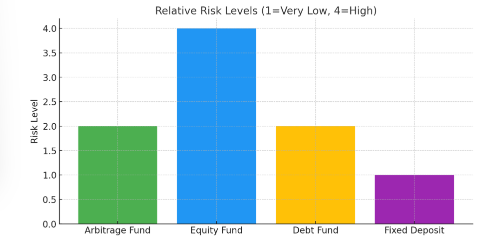
Risk LevelLow–ModerateHighLow–ModerateVery Low
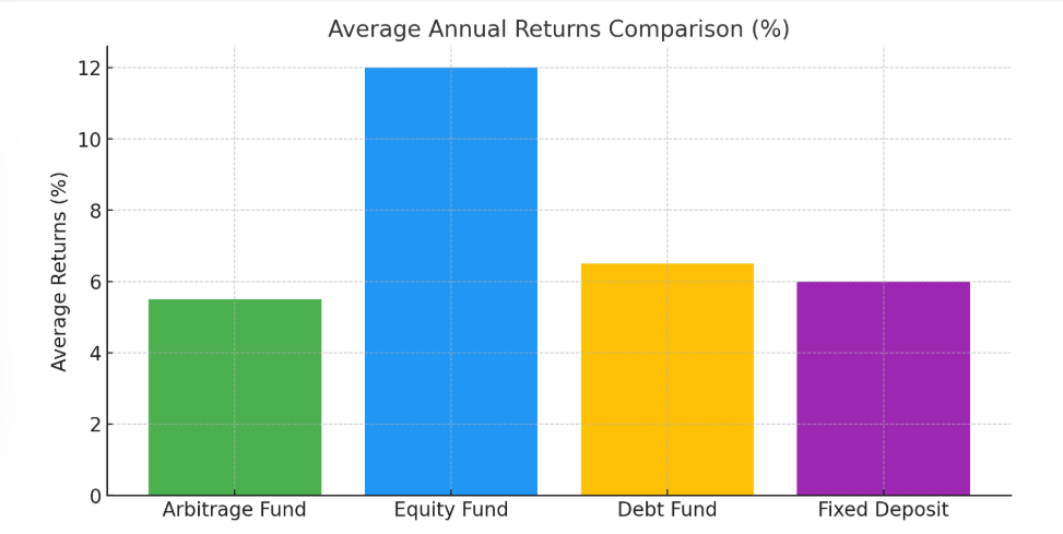
Return Potential4–7% (linked to arbitrage opportunities)High (10–15%+ in long term, but volatile)5–8% (depends on interest rate cycle)5–7% (fixed depending on tenor)
Best Use CaseShort-term parking of fundsLong-term wealth creationMedium-term income & stabilitySafe savings, capital protection
LiquidityHigh (T+1 or T+2 redemption)High (but market risk)HighMedium (premature withdrawal penalty)
Taxation – STCG20% (if held < 12 months)20% (if held < 12 months)taxed at income slabInterest taxed at income slab
Taxation – LTCG12.5% above ₹1.25 lakh (if held > 12 months)12.5% above ₹1.25 lakh (if held > 12 months)20% with indexation (if held > 3 yrs)No LTCG; interest always taxed
Safety of CapitalRelatively safe (but not guaranteed)Market dependentSafer than equity, but credit risk possibleGuaranteed by bank (up to ₹5 lakh insured per depositor)
Expense RatioHigh (due to frequent trades)ModerateLow–ModerateNone
Who Should Invest?Conservative investors seeking better-than-FD short-term returnsAggressive investors with long-term horizonConservative to moderate investors looking for stable returnsRisk-averse investors wanting fixed guaranteed income

Visual Comparisons

Average Returns Comparison (%)

Relative Risk Levels (1=Very Low, 4=High):

Summary:

  • Arbitrage Funds → Good for short-term (low-risk, tax-efficient).
  • Equity Funds → Best for long-term wealth creation.
  • Debt Funds → Balanced choice for medium-term safety + returns.
  • FDs → Safe but least tax-efficient.

In short: Arbitrage funds are low-risk, tax-efficient short-term options but not for long-term growth.